Lorenz attractor with Python

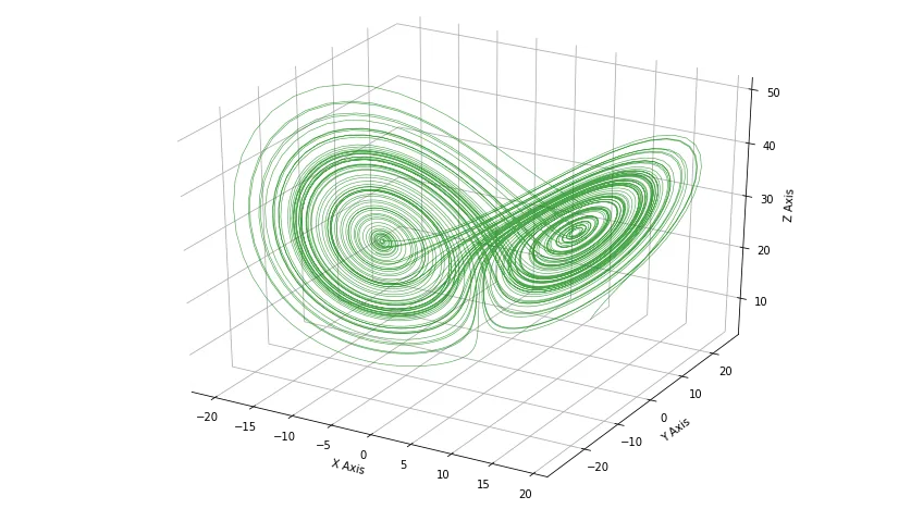
Imagine a world where even the smallest butterfly can destroy the whole planet. It sounds ridiculous, right? However, there may be some truth in it. In the mid-twentieth century the mathematician Edward Lorenz developed a simple mathematical model of atmospheric convection. The model contains a system of three ordinary differential equations which we now know as the Lorenz equations:

$$\begin{aligned} \frac{dx}{dt} &= \sigma (y - x) \\ \frac{dy}{dt} &= x (\rho - z) - y \\ \frac{dz}{dt} &= x y - \beta z \end{aligned}$$

These equations show that if we change the initial conditions even a little bit, we get a different output. Here is the tricky part: the output is fundamentally different, not just slightly off. This behaviour is called chaotic and it is the reason why many physical systems are fundamentally unpredictable.

Solving the Lorenz system #

There are many methods to solve this system. We will use the easiest one, the Euler method. First let us understand how it works on the equation

$$y' = y, \quad y(0) = 1$$

The formula is

$$y_{n+1} = y_n + h f(t_n, y_n)$$

where $h$ is the step. With $h = 1$:

$y_1 = y_0 + h f(y_0) = 1 + 1 \cdot 1 = 2$, $y_2 = 2 + 1 \cdot 2 = 4$, $y_3 = 8$, $y_4 = 16$.

Now we apply the same idea to the Lorenz system:

import numpy as np
import matplotlib.pyplot as plt

sigma, rho, beta = 10, 28, 8 / 3
h, t = 0.01, 10000

x = np.empty(t + 1); y = np.empty(t + 1); z = np.empty(t + 1)
x[0], y[0], z[0] = 10, 10, 10

for i in range(t):
    x[i + 1] = x[i] + h * (sigma * (y[i] - x[i]))
    y[i + 1] = y[i] + h * (x[i] * (rho - z[i]) - y[i])
    z[i + 1] = z[i] + h * (x[i] * y[i] - beta * z[i])

fig = plt.figure(figsize=(12, 9))
ax = fig.add_subplot(projection="3d")
ax.plot(x, y, z, color="g", alpha=0.7, linewidth=0.5)
plt.show()

Sensitivity to initial conditions #

Run the same loop for three starting points that differ by $10^{-5}$ and the trajectories separate after a few seconds of simulated time:

The divergence grows roughly exponentially. A simple chart of the distance between two such trajectories:

How the pieces fit together:

flowchart LR
  A[Initial conditions] --> B[Euler step]
  B --> C{t < T?}
  C -- yes --> B
  C -- no --> D[Plot with matplotlib]